This page was generated from notebooks/mesonic-mbs.ipynb.

Model-Based Sonification using mesonic

This notebooks shows how a Model-Based Sonification can be implemented using mesonic.

import mesonic

from pyamapping import db_to_amp, linlin

import numpy as np
from scipy.spatial import ConvexHull
from scipy.spatial.distance import cdist

import matplotlib.pyplot as plt
import seaborn as sns

Preparation of Synths

Lets start by preparing our Context and Synths.

context = mesonic.create_context()

Starting sclang process... Done.
Registering OSC /return callback in sclang... Done.
Loading default sc3nb SynthDefs... Done.
Booting SuperCollider Server... Done.

context.enable_realtime()

Playback(time=0.00046825408935546875, rate=1)

The model we use allows to interact with it using the mouse.

For this we create a additional SynthDef as a click marker.

context.synths.add_synth_def("noise", r"""
{ |out=0, freq=2000, rq=0.02, amp=0.3, dur=1, pos=0 |
    Out.ar(out, Pan2.ar(
        BPF.ar(WhiteNoise.ar(10), freq, rq)
        * Line.kr(1, 0, dur, doneAction: 2).pow(4), pos, amp));
}""")

'noise'

test = context.synths.create("noise", mutable=False)

test.start()

Data Preparation

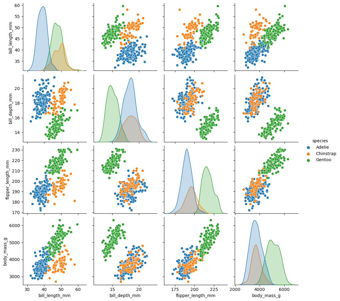
We also prepare the data for the sonification.

We will use the Palmer penguins dataset for the examples.

df = sns.load_dataset("penguins")
df = df.dropna(subset=["bill_length_mm", "bill_depth_mm", "flipper_length_mm", "body_mass_g", "sex"])
df = df.reset_index(drop=True)
df

	species	island	bill_length_mm	bill_depth_mm	flipper_length_mm	body_mass_g	sex
0	Adelie	Torgersen	39.1	18.7	181.0	3750.0	Male
1	Adelie	Torgersen	39.5	17.4	186.0	3800.0	Female
2	Adelie	Torgersen	40.3	18.0	195.0	3250.0	Female
3	Adelie	Torgersen	36.7	19.3	193.0	3450.0	Female
4	Adelie	Torgersen	39.3	20.6	190.0	3650.0	Male
...	...	...	...	...	...	...	...
328	Gentoo	Biscoe	47.2	13.7	214.0	4925.0	Female
329	Gentoo	Biscoe	46.8	14.3	215.0	4850.0	Female
330	Gentoo	Biscoe	50.4	15.7	222.0	5750.0	Male
331	Gentoo	Biscoe	45.2	14.8	212.0	5200.0	Female
332	Gentoo	Biscoe	49.9	16.1	213.0	5400.0	Male

333 rows × 7 columns

%matplotlib inline

sns.pairplot(data=df, hue="species")

<seaborn.axisgrid.PairGrid at 0x256a67e7550>

Data Sonogram

The DataSonogram implements a Data Sonogram

• The model gets a dataset which is plotted in two dimensions.

• Imagine that for each point in the provided dataset a spring is created.

• The data label of the point defines the stiffness of the spring.

• When the user clicks into the plot a shock wave (signaled by noise Synth) is created from the nearest data point.

• The shock wave excites the springs as it is spreading.

• The resulting sonification can reveal clusters.

More details about the Data Sonogram and Model-Based Sonification in general can be found in the corresponding Sonification Handbook Chapter

class DataSonogram:

    def __init__(self, context, df, x, y, label, max_duration=1.5, spring_synth="s1", trigger_synth="noise"):
        self.context = context

        #prepare synths
        self.trigger_synth = context.synths.create(trigger_synth, mutable=False)
        self.spring_synth = context.synths.create(spring_synth, mutable=False)

        # save dataframe
        self.df = df
        self.numeric_df = df.select_dtypes(include=[np.number])

        # check if x and y are valid
        allowed_columns = self.numeric_df.columns
        assert x in allowed_columns, f"x must be in {allowed_columns}"
        assert y in allowed_columns, f"y must be in {allowed_columns}"

        # prepare data for model
        self.labels = self.df[label]
        self.unique_labels = self.labels.unique()
        label2id = {label: idx for idx, label in enumerate(self.unique_labels)}
        self.numeric_labels = [label2id[label] for label in self.labels]
        self.xy_data = self.numeric_df[[x,y]].values
        self.data = self.numeric_df.values

        # get the convex hull of the data
        hull = ConvexHull(self.data)
        hull_data = self.data[hull.vertices,:]
        # get distances of the data points in the hull
        hull_distances = cdist(hull_data, hull_data, metric='euclidean')
        self.max_distance =  hull_distances.max()

        # set model parameter
        self.max_duration = max_duration

        # prepare plot
        self.fig = plt.figure(figsize=(5,5))
        self.ax = plt.subplot(111)

        # plot data
        sns.scatterplot(x=x, y=y, hue=label, data=df, ax=self.ax)

        # set callback
        def onclick(event):
            if event.inaxes is None: # outside plot area
                return
            if event.button != 1: # ignore other than left click
                return
            click_xy = np.array([event.xdata, event.ydata])
            self.create_shockwave(click_xy)

        self.fig.canvas.mpl_connect('button_press_event', onclick)

    def create_shockwave(self, click_xy):
        with self.context.now(0.2) as start_time:
            self.trigger_synth.start()
        # find the point that is the nearest to the click location
        center_idx = np.argmin(np.linalg.norm(self.xy_data - click_xy, axis=1))
        center = self.data[center_idx]
        # get the distances from the other points to this point
        distances_to_center = np.linalg.norm(self.data - center, axis=1)
        # get idx sorted by distances
        order_of_points = np.argsort(distances_to_center)
        # for each point create a sound using the spring synth
        for idx in order_of_points:
            distance = distances_to_center[idx]
            nlabel = self.numeric_labels[idx]
            onset = (distance / self.max_distance) * self.max_duration
            with self.context.at(start_time + onset):
                self.spring_synth.start(
                    freq = 2 * (400 + 100 * nlabel),
                    amp = db_to_amp(linlin(distance, 0, self.max_distance, -30, -40)),
                    pan = [-1,1][int(self.xy_data[idx, 0]-click_xy[0] > 0)],
                    dur = 0.01,
                    info = {"label": self.labels[idx]},
                )

To interact with the plot we use the matplotlib widget

%matplotlib widget

The x and y value can be setted to one of the numeric columns of the data set

numeric_columns = ['bill_length_mm', 'bill_depth_mm', 'flipper_length_mm', 'body_mass_g']

Create two views of the model with different x and y value

dsg1 = DataSonogram(context, df, x="flipper_length_mm", y="body_mass_g", label="species")

dsg2 = DataSonogram(context, df, x="bill_length_mm", y="bill_depth_mm", label="species")

Filtering the MBS

The MBS can be filtered using the processor.event_filters

• Lets create a helper that provides us with a filter function for the labels

def create_label_filter(allowed):
    def label_filter(event):
        label = event.info.get("label", None)
        if label:
            return event if label in allowed else None
        return event
    return label_filter

filter_chinstrap = create_label_filter(["Chinstrap"])
filter_adelie = create_label_filter(["Adelie"])
filter_gentoo = create_label_filter(["Gentoo"])

Select a filter and click again on the plot to listen to the filtered result.

context.processor.event_filters.append(filter_chinstrap)

context.processor.event_filters.remove(filter_chinstrap)

context.processor.event_filters.append(filter_adelie)

context.processor.event_filters.remove(filter_adelie)

context.processor.event_filters.append(filter_gentoo)

context.processor.event_filters.remove(filter_gentoo)

If you want you can combine the single filters

context.processor.event_filters.append(filter_chinstrap)
context.processor.event_filters.append(filter_adelie)

context.processor.event_filters.remove(filter_chinstrap)
context.processor.event_filters.remove(filter_adelie)

Or create a filter that directly filters both labels

combined_filter = create_label_filter(["Adelie", "Chinstrap"])

• We can also remove the panning from the Events

  • This can help to identify the same point in the two different views

def pan_filter(event):
    if event.data.get("pan", None) is not None:
        event.data["pan"] = 0
    return event

context.processor.event_filters.append(pan_filter)

Setting the filter to an empty list [] will reset it

context.processor.event_filters = []

context.close()

Quitting SCServer... Done.
Exiting sclang... Done.